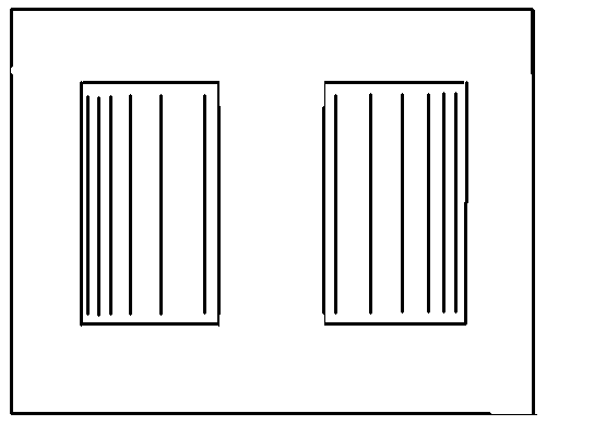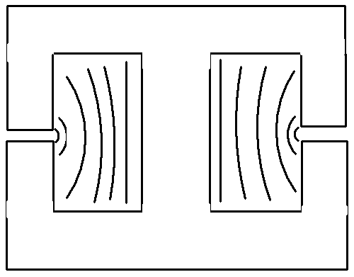

Maxwell field analysis software was used to obtain the values of the squared field due to current in each of the excited windings averaged over the volume of each of the windings in the inductor or transformer, as explained in the instructions on using an external field simulation. The user inputs the values obtained from the simulation in to the Litzopt file. The user then reruns Litzopt to optimize the strand diameter and number considering cost and loss. Litzopt produces a plot of design alternatives and presents a table of costs and losses for each alternative.
1) After you have successfully downloaded Litzopt and set its directory on the Matlab path, run Litzopt from the Matlab command window by typing 'litzopt'.2) You will be prompted to select the type of field geometry to be considered. 1-D and 2-D field calculations are the most computationally efficient and can be used in situations where it is adequate to consider the field in either one or two spatial dimensions. Users optimizing a transformer considering 3-D field effects are required to provide winding volume and magnetic field data from a magnetostatic numerical simulation. This requirement will be removed in future versions of Litzopt.
3) Select the file name at the prompt (you will be allowed to save in the location of your choice).
4) Choose to edit your file immediately or edit it later.
1) Using any text editor, open the text file that has previously been created. To use the Matlab text editor (preferred), open Matlab and select "File", "Open" or double click on the file (pc users).
2) Read the heading and verify that the appropriate number of windings are assigned to your transformer.
3) Replace all the ??'s with the data that is called for. If you are not using the Matlab text editor, these will not appear red. Note that all elements must be replaced for proper operation. If you are presented with a vector with too many or too few elements for your data, you did not select the correct number of windings for your transformer when creating this text file. Create another text file (see step 1). DO NOT insert or omit elements in vectors or matrices as this will lead to undesired program operation. A comprehensive description of each section of code to be edited follows.
a) Room temperature copper is typically the conductive material used in most transformers. This is Litzopt's default resistivity value. If you are not operating with room temperature copper, change the value of 'rhoc' to your resistivity in ohm-meters. Otherwise leave this unchanged.
b) AWG (American Wire Gauge) strand sizes 32-48 is a typical range of strand diameters to consider. This is Litzopt's default a range of designs. If you would like to optimize your transformer considering a range of strand diameters other than these, change the value of 'awg' to your range of strand sizes. Otherwise leave this unchanged.
c) Enter the dimensions of the core and bobbin window in meters. This includes the breadth of the core window, the height of the core window, the breadth of the bobbin window and the height of the bobbin window. The dimensions are shown in Figure 1.
Figure 1: Core and Bobbin Window Dimensions
d) Enter the length of the air gap in the magnetic core in meters. If the component has no gaps in the core, enter zero for the gap length.
e) Enter the maximum achieveable packing factor, which indicates the density of wire that can be achieved in manufacturing the component.
f) Enter the average turn length of each of your windings. For a cylindrical winding (around a round center post), this can be found by computing the radius from the center of the core to the center of the given winding, shown in Figure2, by 2
.
breadth of core centerpost radius winding distance to core half winding width radius of average turn length
Figure 2: A typical winding window inside a core.
g) Users opting to select the automatic 2-D field solution are required to enter the width (horizontal) and height (vertical) dimensions of the winding cross-sections (with the horizontal measured in the bw direction). Also, the cartesian coordinates of the cross-section centers (x,y) are to be entered with the origin at the bottom left corner of the winding window. These dimensions can be seen in Figure 3.
Figure 3: The cross-section of a typical rectangular transformer windingh) The current waveform data is to be entered as piece-wise linear with values preceding each of the time segments. Enter the length of each of your time segments. It is assumed that your segments are periodic and that your last time segment immediately precedes the first.
i) The current data required consists of a vector of current values for each of the transformer windings. Each of the vector contains the data for a specific winding. A given vectors elements represent current values in that winding at the beginning of each of the time segments. The first entry is the starting value for the first time segment. The remaining entries will describe the current waveform in a piece-wise linear manner. The final entry in the vector represents the current value at the beginning of the final time segment, and the current value at the end of the final time segment is assumed to return to that at the beginning of the first time segment (given by the first term of the vector). Sinusoidal excitation can be implemented by computing values in the data file (click here to see an example).
j) Number of turns in each winding.
k) Users wishing to evaluate the original design which is to be optimized by litzopt, must enter the original wire size for each winding and the original number of strands for each winding. Leave these values set to zero if this function is not desired.
l) Users opting to select the 1-D option are required to provide the area of the bobbin window in meters squared.
m) Users opting to select the 3-D option are required to provide volume data that consists of a single vector with an entry for each transformer winding. The total volume occupied by each of the windings is to be inputted. The volume of a transformer winding can be approximated by the rectangular area shown in Figure 3 multiplied by the average length of a turn. This is not required for 1-D and 2-D optimizations. The volume occupied by the winding is defined as the space occupied by conductive material and the immediate vicinity, as in Figure 3.n) Users opting to select the 3-D option are required to provide magnetic field data from a magnetostatic finite element simulation (e.g. Maxwell). This requires following the winding excitation sequence given in your data file and obtaining the volume integral of the squared magnetic flux density (B) in each winding for each specified excitation. All excited windings are to be considered with unit (NI = 1 ampere) excitation. The excitation sequence includes all combinations of one and two winding excitation. A sample excitation sequence is available here. The data entry process is completed when all the ??'s have been replaced by spatial integral of squared field values. Note that users who selected the 1-D and 2-D optimizations will not be presented with entries to be edited for magnetic field data as Litzopt computes the required field data analytically. A more detailed description of how to obtain the squared flux density data is available here.4) When editing is complete and no question marks appear, save your file.
1) Run Litzopt from the Matlab command window.2) Select "Existing" and select the file you have edited.
3) A table of designs appears in the Matlab command window.
4) Three figures appear. The first shows the current waveforms in each winding with respect to time (the user should verify that they are the proper current waveforms); the second figure is a curve of cost and loss of optimal designs. The final figure displays the locations and dimensions of the winding cross-sections in the winding window (the user should verify that the windings are the proper sizes and locations).See an example.