Compatible Data Files

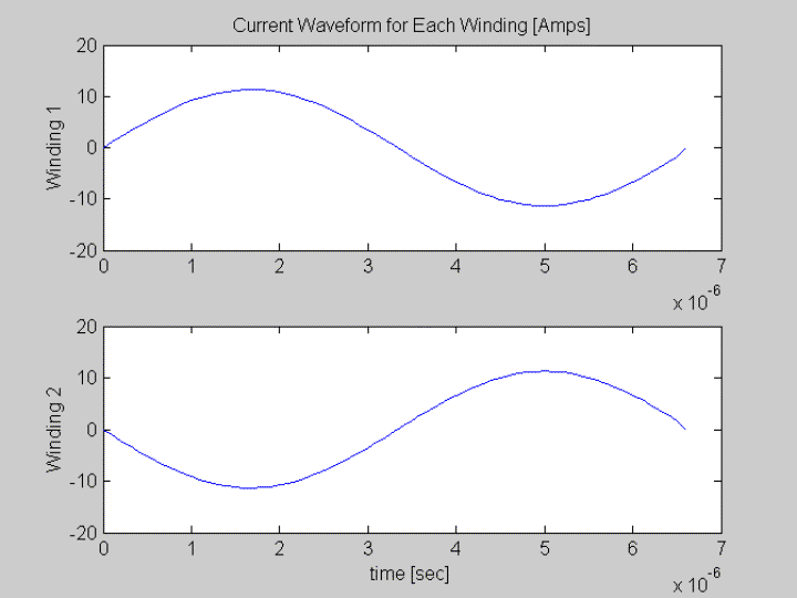
A typical data file is shown below for a two-winding, 30-turn to 30-turn transformer on an EC-70 ferrite core with sinusoidal excitation of 150 kHz and 8 A rms in both windings.  Both transformer windings are of the same size.  The core is gapless and has a window breadth of  44.6 mm; the bobbin allows a winding  area of 41.5 mm by 24 mm high; each of the two windings may then take up a height of 12 mm. The field geometry is considered in one spatial dimension.   Note the code used for the sinusoidal excitation.   All generated text appears in green and data entered into the generated data file is displayed in red.  Data that is optional to change appears in blue.

%For an example and help, go to www.thayer.dartmouth.edu/inductor/litzopt or refer to winding data for use with litzopt.%Please replace the question marks with the pertinent data and leave all else alone....

%There are 2 windings in your transformer.

%Resistivity (1.77e-8 is for room temperature copper)
  rhoc =1.77e-8; % [ohm-meters]

%Perform optimization on designs with wire sizes ranging from American Wire Gauge strand size (32 to 48 is the default)
  awg = [32:2:48]; %

%Average turn length for each winding ... 2 elements are required in this vector.
  len =[ 97.3e-3 97.3e-3];  %

%Duration of each time segment ... 100 elements are required in this vector.
    divisions=100;
    f=150e3; % 150 Khz
    period=1/f;
    inc=period/divisions;
    dt =inc*ones(1,divisions);

%Current at the end of the last interval is assumed equal to the first current value.

 %Current values for winding 1 at the beginning of each time segment ... 101 elements are required in this
    vector.

  A=8*sqrt(2); % Waveform Amplitude
  t=[0:inc:period-inc];
  w=2*pi*f;
  I(1,:)=A*sin(w.*t);

%Current at the end of the last interval is assumed equal to the first current value.

 %Current values for winding 2 at the beginning of each time segment ... 101 elements are required in this
    vector.
 I(2,:)= -I(1,:);

%Number of turns in each winding... 2 elements are required in this vector.
   N=[ 30 30]; %[turns]
%Breadth of the winding window in meters.
  bw=0.0446;
  gap='No Gap';


The output of Litzopt, run with the above data file, is a set of figures (below), as well as a table of costs, losses, and stranding (below).  The first figure is a plot of the current waveforms with respect to time.  The user can examine this figure to ensure that current waveform data has been correctly entered.  The next figure generated by Litzopt is the 'optimal design frontier'.  Each point on the figure describes a distinct stranding design  with a particular wire size, strand number for each winding, cost, and loss.  Designs on the curve yield the lowest loss at the given cost.  Improving the performance of a transformer from a design on the optimal design frontier requires upgrading to a more costly stranding design.   All the designs have costs relative the Awg 44 design (i.e. Awg 44 has a relative cost of unity). 


Gauge      Cost(rel)         Loss [W]         Number of Strands for Winding  1      Number of Strands for Winding  2
32           0.03059           42.57                         5.051                                                    5.051
34           0.04906           27.91                         12.53                                                    12.53
36           0.07962           18.56                         30.96                                                    30.96
38           0.1327             12.53                         76.53                                                    76.53
40           0.2331             8.602                        190.4                                                    190.4
42           0.4485             6.084                         473.3                                                    473.3
44           1                      4.515                         1130                                                     1130
46           2.824               3.489                         2508                                                     2508
48           10.44               2.744                         5253                                                     5253


A typical data file is shown below for a 7-turn to 49-turn gapped flyback transformer core with a triangular excitation of 260 kHz with 11.4 A peak current in the primary winding and 1.6 A peak current in the secondary winding (further detail is available regarding this transformer here).   The integral of B squared values are obtained from an external simulations.    All generated text appears in gray and data entered into the generated data file is displayed in red.  Data that is optional to change appears in blue.

%For an example and help, go to www.thayer.dartmouth.edu/inductor/litzopt, or refer to winding data for use with litzopt.

%Please replace the question marks with the pertinent data and leave all else alone....

%There are 2 windings in your transformer

%Resistivity (1.77e-8 is for room temperature copper)
  rhoc =1.77e-8; % [ohm-meters]

%Perform optimization on designs with wire sizes ranging from American Wire Gauge strand size (32 to 48 is the default)
  awg = [32:2:48]; %

%Average turn length for each winding...
  len =[ 3.79e-2 5.08e-2 ];  %[meters]
 

  %Duration of each time segment ... 3 elements are required in this vector
  dt = [3.8e-6 .07e-6 3.9e-6];

%Current values for winding 1 at the beginning of each time segment ... 3 elements are required in this vector.
I(1,:)=[0 11.4 0 ];

%Current at the end of the last interval is assumed equal to the first current value

 %Current values for winding 2 at the beginning of each time segment
   I(2,:)=  [0 0 -11.4/7 ]; %[amperes]

%Volume of each winding...
  vol=[ 0.0821    0.2480 ].*1e-5; %[cubic meters]

%Number of turns in each winding...
  N=[ 7 49   ];  %[turns]

%Integral of Bsquared values from simulation with current in winding 1

       % Enter integral of B squared  over winding 1
       int_B2(1,1,1)=7.3875e-015; %[T^2-m^3 ]
       % Enter integral of B squared  over winding 2
       int_B2(1,1,2)=2.7289e-015; %[T^2-m^3 ]

%Integral of B squared values from simulation with current in winding 1 and 2

       % Enter integral of B squared  over winding 1
       int_B2(1,2,1)=  1.3110e-015%[T^2-m^3 ]
       % Enter integral of B squared  over winding 2
       int_B2(1,2,2)=3.3920e-015; %[T^2-m^3 ]

%Integral of Bsquared values from simulation with current in winding 2

       % Enter integral of B squared  over winding 1
       int_B2(2,2,1)=1.0290e-014; %[T^2-m^3 ]
       % Enter integral of B squared  over winding 2
       int_B2(2,2,2)=6.4625e-015; %[T^2-m^3 ]


The output of Litzopt, run with the above data file, is a set of figures (below), as well as a table of costs, losses, and stranding (below).  The first figure is a plot of the current waveforms with respect to time.  The user can examine this figure to ensure that current waveform data has been correctly entered.  The next figure generated by Litzopt is the 'optimal design frontier'.  Each point on the figure describes a distinct stranding design that can be associated with a particular wire size, strand number for each winding, cost, and loss.  Designs on the curve yield the lowest loss at the given cost.  Improving the performance of a transformer from a design on the optimal design frontier requires upgrading to a more costly stranding design.  All the designs have costs relative the Awg 44 design (i.e. Awg 44 has a relative cost of unity).


Gauge    Cost(rel)         Loss [W]         Number of Strands          Number of Strands
                                                             for Winding  1                 for Winding  2

32         0.03059       5.942                   0.5236                             0.1585
34         0.04906       3.896                   1.299                               0.3932
36         0.07962       2.591                   3.209                               0.9715
38         0.1327        1.749                   7.933                               2.402
40         0.2331         1.201                   19.74                               5.975
42         0.4485         0.8492                 49.06                               14.85
44         1                  0.6302                 117.2                               35.47
46         2.824           0.487                   260                                  78.71
48         10.44           0.383                   544.5                               164.8